Stochastic Simulations

This vignette demonstrates how to use the simulate method for calculating k-step-ahead stochastic simulations trajectories.

Introduction

Notation

We use subscript $x_{t} = x(t)$ to denote time for continuous variables.
We use subscript $y_k = y(t_k)$ to indicate discrete time-points for discrete variables.
We denote the set of observations from the initial time $t_0$ until the “current” time $t_{i}$ by $\mathcal{Y}_{i} = \left\{ y_{i}, y_{i-1},...,y_{1},y_{0} \right\}$
We denote mean and variance by $\mu_{t} = \mathrm{E}\left[x_t\right]$ and $P_{t} = \mathrm{V}\left[x_t\right]$ .
We use $\mu_{k \mid k-1}$ and $P_{k \mid k-1}$ to denote the mean/variance at time $t_{k}$ conditional on the observations $\mathcal{Y}_{k-1}$ i.e. $\mu_{k \mid k} = \mathrm{E}\left[x_{t_k} \mid \mathcal{Y}_{k}\right] \qquad\qquad P_{k \mid k} = \mathrm{V}\left[x_{t_k} \mid \mathcal{Y}_{k}\right]$

Stochastic State Space System

We consider the following types of stochastic state space systems

$x_{t} = f(t,x_t,u_t,\theta) \, \mathrm{d}t + G(t,x_t,u_t, \theta) \, \mathrm{d}\mathrm{d}B_{t}$

$y_{k} = h(t_k, x_{t_k}, u_{t_k}, \theta) + \varepsilon_{k}$

where the observation noise is zero-mean Gaussian $\varepsilon_{k} \sim \mathcal{N}(0,\Sigma(t_k, x_{t_k}, u_{t_k}, \theta))$ . In this notation $u$ are inputs and $\theta$ are fixed effects parameters to be estimated.

We refer to the functions $f$ as the drift, $G$ as the diffusion, and $h$ as the link. We may omit arguments and just write e.g. $f(x_t)$ for readability.

Observations and Likelihood

The likelihood, which is the joint density of all observations, can be rewritten by using repeated conditioning as

$L(\theta) = p(\mathcal{Y}_{N}) = \prod_{k=1}^{N} p(y_{k} \mid \mathcal{Y}_{k-1}) = \prod_{k=1}^{N} p(h(x_{k}) + \varepsilon_{k} \mid \mathcal{Y}_{k-1})$

What is a “Simulation”?

When we say a stochastic simulation(s) we mean sample trajectories drawn from the joint state distribution at all future sampling times conditional on the (relative) initial posterior state distribution i.e.

$\mathcal{X}_{t_{i+k}} = \left( x_{t_i}, x_{t_{i+1}}, \dots, x_{t_{i+k-1}}, x_{t_{i+k} } \right) \mid \, p(x_{t_i})$

The initial distribution $p_{X_{t_i}}$ is approximated by a Gaussian with mean and covariance given by the posterior expectation and covariance i.e.

$X_{t_{i}} \sim N(\hat{x}_{i|i}, P_{i|i} )$

We may sample such trajectories as follows:

Sample from $p(x_{t_i})$ to generate $X_{t_{i}}$ .
Use the Euler-Maruyama method to generate the future state values iteratively

The Euler-Maruyama discretization for the SDE is given by

$X_{t_{j+1}} = X_{t_{j}} + f(X_{t_{j}},u_{t_{j}},t_{j}) \, \Delta t_{j} + G(X_{t_{j}},u_{t_{j}},t_{j}) \, \Delta B_{j}$

for $j = i, ... , i+k-1$ , and where $\Delta B_{j} \sim N(0,\Delta t_{j})$ .

Algorithm

When using the simulate method the forecast horizon is controlled by the k.ahead argument, i.e. how many time-steps “into the future” forecasts are wanted for.

The algorithm returns $N$ forecast scenarios, calculated by nrow(data)-k.ahead. Each of these $i=0,1,..,N$ scenarios consist of $k_{\text{ahead}}+1$ state values, for every $n_{\text{sims}}$ requested simulation trajectories, one for each time point $t=t_{i+j}$ where $j=0,1,..,k_{\text{ahead}}$ . The number of simulation trajectories $n_{\text{sim}}$ can be controlled via the n.sims argument.

The algorithm carries out the following step-wise procedure:

Filter with the provided data to obtain posterior state and covariance estimates for every point in time in the provided data[,"t"] column.
Extract the first $N$ estimates and discard the remainder.
For each $i=0,1,..,N$ sample $k=0,1,..,n_{\text{sims}}$ realisations $X^{(k)}$ from the posterior Gaussians given by

$X^{(k)} \sim \mathcal{N}\left(\hat{x}_{i \mid i}, P_{i \mid i}\right)$

For each of the realized variables $X^{(k)}$ apply the Euler-Maruyama scheme repeatedly until from the initial time $t_{i}$ until time $t_{i+k_{\text{ahead}}}$ producing forecasts at each of the intermediate times $t_{i+j}$ .

In summary this produces for each of the system states (i.e. for each element of $x_t$ ) a list with $N$ entries, where each entry is a matrix of $k_{\text{ahead}}+1$ rows and $n_{\text{sims}}$ columns. Each column is thus a stochastic realisation of the associated forecast distribution.

Example

We consider a modified Ornstein Uhlenbeck process:

$\begin{align} \mathrm{d}x_{t} & = \theta (a_t - x_{t}) \, \mathrm{d}t \, + \sigma_{x} \, \mathrm{d}b_{t} \\ y_{t_{k}} & = x_{t_{k}} + \varepsilon_{t_{k}} \end{align}$

where the mean is given by (some time-varying input)

$a_t = tu_{t}^{2}-\cos(tu_{t})$

and $u_{t}$ is a known input signal. The variance is zero-mean Gaussian $\varepsilon_{t_{k}} \sim \mathcal{N}(0,\sigma_{y}^2)$ , and we assume that $\sigma_{y}$ is known.

Create Model

First we create the model as follows:

## Load libraries
library(ctsmTMB)
library(ggplot2) ## plots

## Create model
model <- newModel()
model$addSystem(dx ~ theta * (t*u^2-cos(t*u) - x) * dt + sigma_x*dw)
model$addObs(y ~ x)
model$setVariance(y ~ sigma_y^2)
model$addInput(u)

## Set parameter values
## note: not strictly necessary to set lower/upper bounds
model$setParameter(
  theta   = c(initial = 2, lower = 0,    upper = 100),
  sigma_x = c(initial = 0.2, lower = 1e-5, upper = 5),
  ## fix sigma_y to 0.05 by not giving any upper/lower bounds
  sigma_y = c(initial = 5e-2)
)

## Set initial state mean and covariance
## note: diag(1) is not strictly needed
model$setInitialState(list(1, 1e-1*diag(1)))

Create Data

Next we create a data.frame that contains time-points and input values.

## set true parameters, and create data
true.pars <- c(theta=20, sigma_x=1, sigma_y=0.05)
dt.sim <- 1e-3
t.sim <- seq(0, 1, by=dt.sim)

## seed for input creation
set.seed(20)
u.sim <- cumsum(rnorm(length(t.sim),sd=0.1))
df.sim <- data.frame(t=t.sim, y=NA, u=u.sim)

Simulate

Then we call the method to simulate.

## Set rng seeds for C++ states and observations
cpp.seeds <- c(20,20)

## perform simulation
sim <- model$simulate(data=df.sim, 
                      pars=true.pars, 
                      k.ahead = nrow(df.sim)-1, ## default
                      n.sims = 2,
                      cpp.seeds = cpp.seeds)
## Checking model components...
## Compiling C++ function pointers...
## Checking and setting data...
## Simulating with C++...
## Returning results...
## Finished.

A few notes for the code above:

We use the default value of argument k.ahead = nrow(data)-1 to get a forecast over the entire time-vector. This means that there is only $N=1$ forecast scenario.
We remove the first observation to prevent a posterior update at the initial time-point t[1]. This allows us to fully control the initial state mean and covariance via setInitialState.
Since k.ahead = nrow(data)-1 and $N=1$ implies just one forecast scenario starting from the initial time point the remaining observations y[2:nrow(data)] will not be used, why we set them as NA.
The cpp.seeds argument control the RNG seed for the state and observations respectively, i.e. for the Brownian increments $dB_t$ and for the observation noise $\varepsilon_t$ .

Output

The returned sim object is a list of lists of lists of matrices.

The outer list has the three elements states, observations and times.
The states, and observations list each contain entries for all state and observation variables respectively named accordingly.
The state and observation variable lists e.g. x, y contain matrices where the columns are simulated forecast trajectories, and the rows corresponds to forecast time-points, as described in the Algorithm Overview section. These are named i0, i1, i2 indicative of the time-point from which the forecast begun.
Each entry in the ‘times’ list contains 5-column matrices with time indices and time-values for each of the forecast scenarios. These are also named i0, i1, i2 matching those from the states and observations.

Below we bind together the matching output from times, states$x, observations$y for the first (and only in this case) forecast scenario.

mat <- as.matrix(data.frame(sim$times$i0, x=sim$states$x$i0, y=sim$observations$y$i0))
head(mat)
##      i j t.i   t.j k.ahead       x.1       x.2       y.1       y.2
## [1,] 0 0   0 0.000       0 0.5255843 0.7101432 0.4505726 0.6643129
## [2,] 0 1   0 0.001       1 0.5018194 0.7004629 0.5124870 0.7392365
## [3,] 0 2   0 0.002       2 0.5349053 0.6775028 0.6347102 0.6949730
## [4,] 0 3   0 0.003       3 0.4575998 0.6020440 0.3839036 0.5357770
## [5,] 0 4   0 0.004       4 0.4585211 0.6045719 0.5060700 0.6592290
## [6,] 0 5   0 0.005       5 0.4160683 0.5715023 0.3950665 0.5699553
tail(mat)
##         i    j t.i   t.j k.ahead        x.1        x.2        y.1        y.2
##  [996,] 0  995   0 0.995     995 -0.2784495 -0.3005070 -0.2290918 -0.2292191
##  [997,] 0  996   0 0.996     996 -0.2523736 -0.2198851 -0.2605479 -0.1425121
##  [998,] 0  997   0 0.997     997 -0.3046669 -0.2223966 -0.4343075 -0.2722980
##  [999,] 0  998   0 0.998     998 -0.2688731 -0.2173837 -0.2827411 -0.2773187
## [1000,] 0  999   0 0.999     999 -0.1870747 -0.1701929 -0.1368140 -0.1730233
## [1001,] 0 1000   0 1.000    1000 -0.1478336 -0.1148420 -0.1612386 -0.1022415

The column i holds the time-index from where the forecast began.
The column j holds the time-index for where the forecast is.
The column t.i is the numeric time value associated with index i.
The column t.j is the numeric time value associated with index j.
The column k.ahead is the number of forecasted timesteps since the last posterior update (if any data was available at that time-point).

Note that because we chose only a single simulation by setting $n_{\text{sims}}=2$ via the argument n.sims=2 we get two columns (trajectories) for x and y.

Estimating with the Simulated Observations

Let us extract the observations that we just simulated, and feed them to estimate to see if we can recover the true parameters.

## Extract all observations
y.sim <- sim$observations$y$i0[,1]

## Only select every tenth, to reduce the available information
iobs <- seq(1, length(t.sim), by=10)
t.obs <- t.sim[iobs]
y.obs <- y.sim[iobs]
u.obs <- u.sim[iobs]

## Create data for re-estimation
df.obs <- data.frame(
  t = t.obs,
  u = u.obs,
  y = y.obs
)

## Try to estimate the parameters
fit <- model$estimate(df.obs)
## Checking and setting data...
## Constructing objective function and derivative tables...
## Minimizing the negative log-likelihood...
##   0:     942.26752:  2.00000 0.200000
##  10:    -50.890921:  20.1830  1.32382
##   Optimization finished!:
##             Elapsed time: 0.003 seconds.
##             The objective value is: -5.11315e+01
##             The maximum gradient component is: 4.7e-06
##             The convergence message is: relative convergence (4)
##             Iterations: 17
##             Evaluations: Fun: 19 Grad: 18
##             See stats::nlminb for available tolerance/control arguments.
## Returning results...
## Finished!

So that was fairly straight-forward. We can inspect the fit to see the related Wald test statistics.

fit
## Coefficent Matrix 
##         Estimate Std. Error t value  Pr(>|t|)    
## theta   18.96771    2.24401  8.4526 2.549e-13 ***
## sigma_x  1.36329    0.12749 10.6935 < 2.2e-16 ***
## ---
## Signif. codes:  0 '***' 0.001 '**' 0.01 '*' 0.05 '.' 0.1 ' ' 1

Many Simulations

We can change the n.sims argument to get more trajectories, and these can be plotted easily with matplot:

sim <- model$simulate(data=df.sim, pars=true.pars, n.sims=5, cpp.seeds = cpp.seeds)
## Checking and setting data...
## Simulating with C++...
## Returning results...
## Finished.
x <- sim$states$x$i0
t <- sim$times$i0
matplot(t[,"t.j"], x, type="l", lty="solid", ylim=c(-4,4), xlab="Time")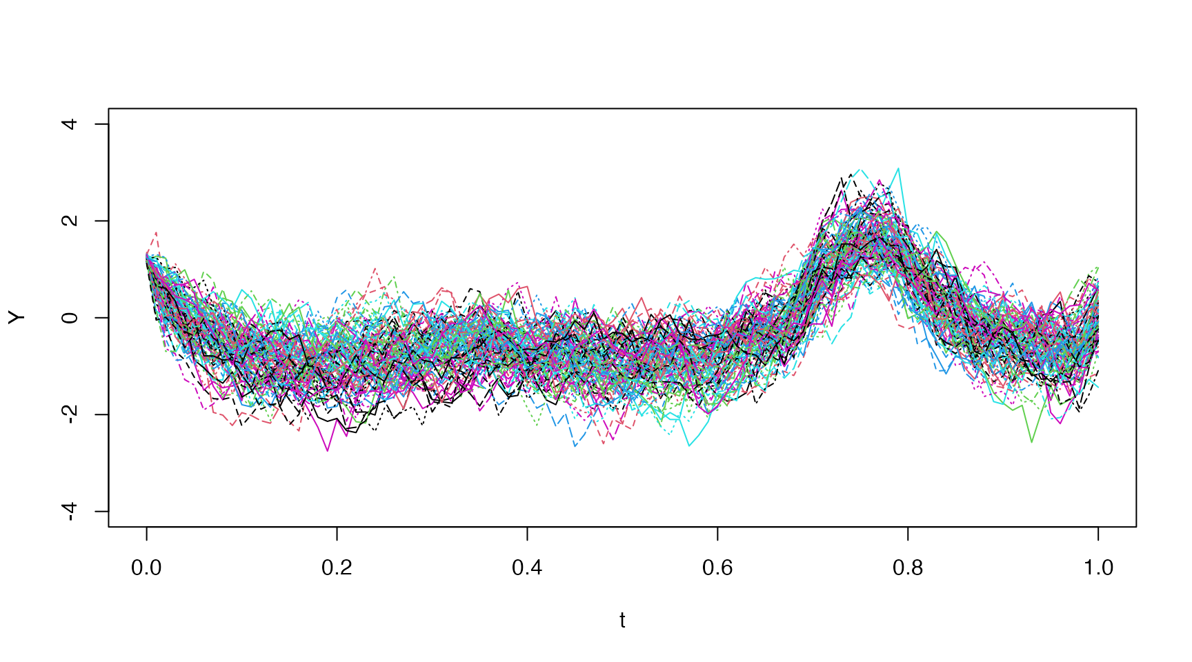

Increasing Process Noise

Let’s check the effect of the process noise by increasing from $\sigma_{x}=1$ up to $\sigma_{x}=4$ .

new.pars <- true.pars
new.pars["sigma_x"] <- 4
sim <- model$simulate(data=df.sim, pars=new.pars, n.sims=5, cpp.seeds=cpp.seeds)
## Checking and setting data...
## Simulating with C++...
## Returning results...
## Finished.
x <- sim$states$x$i0
t <- sim$times$i0
matplot(t[,"t.j"], x, type="l", lty="solid", ylim=c(-4,4), xlab="Time")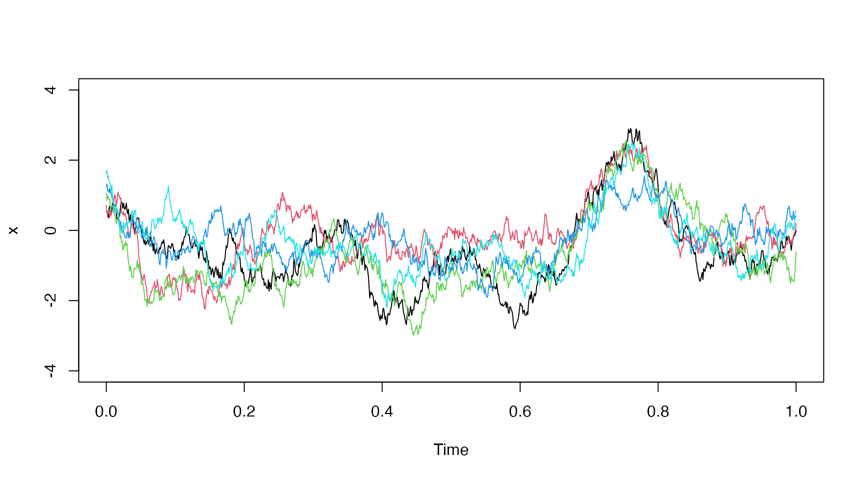

Distribution Plot

We demonstrate how one might plot the entire distribution using ggplot2 below:

new.pars["sigma_x"] <- 4
sim <- model$simulate(data=df.sim, pars=new.pars, n.sims=100, cpp.seeds=cpp.seeds)
## Checking and setting data...
## Simulating with C++...
## Returning results...
## Finished.

## quantiles
p <- c(0.01, 0.05, seq(0.1,0.9,by=0.1), 0.95, 0.99)
Q <- t(apply(sim$states$x$i0, 1,function(x) quantile(x, probs=p)))

## create data for distribution plot
p.center <- p[-length(p)] + diff(p)/2
col.ids <- c(col(Q[,-1]))
row.ids <- c(row(Q[,-1]))
fan.df <- data.frame(
  t = sim$times$i0[row.ids,"t.j"],
  ymin = c(Q[,-ncol(Q)]),
  ymax = c(Q[,-1]),
  ids = col.ids,
  ## symmetric colors around median
  fill.value = abs(0.5 - p.center[col.ids])
)

## Create plot
ggplot() +
  geom_ribbon(data=fan.df, aes(x=t, ymin=ymin, ymax=ymax, fill=fill.value, group=ids)) +
  geom_line(aes(x=sim$times$i0[,"t.j"], y=Q[,"50%"]), color="black", linewidth=0.3) +
  scale_fill_gradientn(colors=c("red","yellow")) +
  coord_cartesian(ylim=c(-4,4)) +
  guides(fill="none") +
  labs(x="Time",y="") +
  theme_minimal()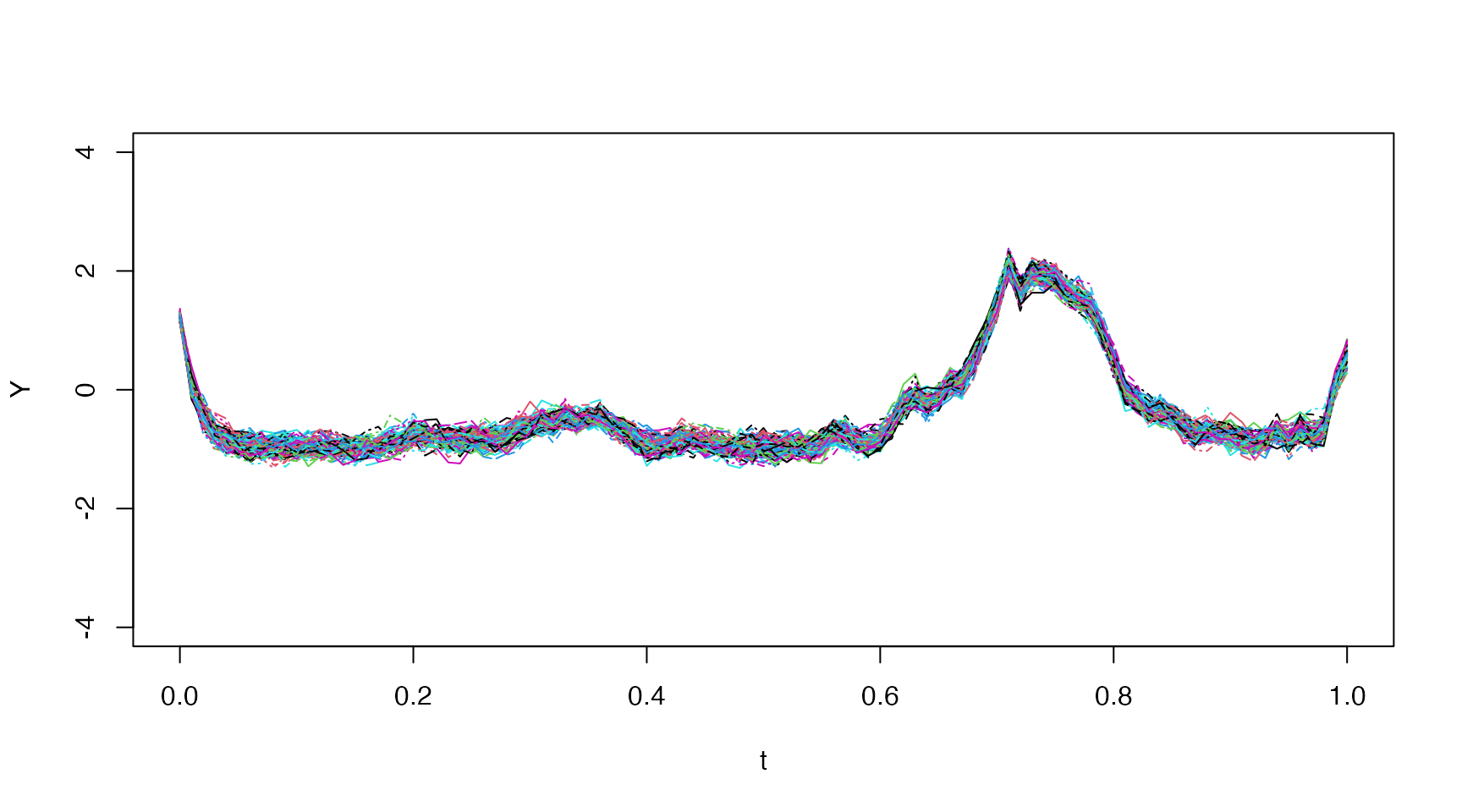

Method Arguments

The simulate method accepts the following arguments

model$simulate(data,
               pars = NULL,
               use.cpp = TRUE,
               cpp.seeds = NULL,
               method = "ekf",
               ode.solver = "rk4",
               ode.timestep = diff(data$t),
               simulation.timestep = diff(data$t),
               k.ahead = nrow(data)-1,
               return.k.ahead = 0:min(k.ahead, nrow(data)-1),
               n.sims = 100,
               ukf.hyperpars = c(1, 0, 3),
               initial.state = self$getInitialState(),
               estimate.initial.state = private$estimate.initial,
               silent = FALSE,
               ...)

`pars`

See the description in the predict vignette.

`use.cpp`

Use C++ or pure R implementation.

See the description in the predict vignette.

`method`

Filtering method used - one of ‘ekf’, ‘lkf’, or ‘ukf’.

See the description in the estimate vignette.

`ode.solver`

See the description in the estimate vignette.

`ode.timestep`

See the description in the estimate vignette.

`k.ahead`

See the description in the predict vignette.

`return.k.ahead`

See the description in the predict vignette.

`simulation.timestep`

The number of intermediate time-steps taken between time-points in the provided data for the Euler-Maruyama method.

`n.sims`

The number of stochastic simulation trajectories generated.

`initial.state`

Sets the initial state $\hat{x}_{0 \mid 0}$ and variance $P_{0 \mid 0}$ .

`estimate.initial.state`

A boolean to indicate whether or not estimate the initial state mean value instead of using the one provided via the model$setInitialState method or the initial.state argument to this method.

The estimation is carried out by root-finding the stationary mean equation equivalent to minimizing

$\hat{x}_{0 \mid 0} = \min_{x} \left(f(t_0, x, u_{0}, \theta)\right)^{2}$

using a Newton approach.

Note: This option is only available when use.cpp=FALSE using the pure R implementation.

`silent`

Disable message print-outs.

Phillip Vetter

2026-02-27

Introduction

Notation

Stochastic State Space System

Observations and Likelihood

What is a “Simulation”?

Algorithm

Example

Create Model

Create Data

Simulate

Output

Estimating with the Simulated Observations

Many Simulations

Increasing Process Noise

Distribution Plot

Method Arguments

`pars`

`use.cpp`

`method`

`ode.solver`

`ode.timestep`

`k.ahead`

`return.k.ahead`

`simulation.timestep`

`n.sims`

`initial.state`

`estimate.initial.state`

`silent`