Plot of k-step predictions from a ctsmTMB prediction object

Usage

# S3 method for ctsmTMB.pred
plot(
  x,
  y,
  k.ahead = unique(x[["states"]][["k.ahead"]]),
  state.name = NULL,
  type = "states",
  against = NULL,
  ...
)

Arguments

x: a ctsmTMB.pred object
y: not used
k.ahead: an integer indicating which k-ahead predictions to plot
state.name: a string indicating which states to plot
type: one of 'states' or 'observations', to plot
against: name of an observations to plot predictions against
...: additional arguments

Value

A plot of predicted states

Examples

library(ctsmTMB)
model <- ctsmTMB$new()

# create model
model$addSystem(dx ~ theta * (mu+u-x) * dt + sigma_x*dw)
model$addObs(y ~ x)
model$setVariance(y ~ sigma_y^2)
model$addInput(u)
model$setParameter(
  theta   = c(initial = 1, lower=1e-5, upper=50),
  mu      = c(initial=1.5, lower=0, upper=5),
  sigma_x = c(initial=1, lower=1e-10, upper=30),
  sigma_y = 1e-2
)
model$setInitialState(list(1,1e-1))

# fit model to data
fit <- model$estimate(Ornstein)
#> Building model...
#> Checking data...
#> Constructing objective function and derivative tables...
#> ...took: 0.09 seconds.
#> Minimizing the negative log-likelihood...
#>   0:     159.30847:  1.00000  1.50000  1.00000
#>   1:     154.15990: 0.826082  1.71820  1.96028
#>   2:     136.01211: 0.614019  2.04466  1.64652
#>   3:     129.29879: 0.625113  2.06221  1.47868
#>   4:     128.42258: 0.666452  2.12632  1.14915
#>   5:     122.27008: 0.825282  2.37200  1.31892
#>   6:     106.61489:  1.59116  3.48574  1.25982
#>   7:     101.72505:  2.18624  3.49501  1.18917
#>   8:     99.610055:  2.43782  3.00283 0.957522
#>   9:     91.160123:  3.00760  2.93833  1.13182
#>  10:     87.333934:  3.60427  2.95994  1.07975
#>  11:     86.392347:  3.62036  3.05856  1.06026
#>  12:     85.804273:  4.02690  3.03800  1.04788
#>  13:     85.776558:  4.04412  3.02977  1.06498
#>  14:     85.771776:  4.04182  3.03209  1.06035
#>  15:     85.771772:  4.04188  3.03208  1.06018
#>  16:     85.771772:  4.04186  3.03210  1.06019
#>  17:     85.771772:  4.04186  3.03210  1.06019
#> 	 Optimization finished!:
#>             Elapsed time: 0.006 seconds.
#>             The objective value is: 8.577177e+01
#>             The maximum gradient component is: 2.7e-05
#>             The convergence message is: relative convergence (4)
#>             Iterations: 17
#>             Evaluations: Fun: 25 Grad: 18
#>             See stats::nlminb for available tolerance/control arguments.
#> Returning results...
#> Finished!

# perform moment predictions
pred <- model$predict(Ornstein)
#> Checking data...
#> Predicting with R...
#> Returning results...
#> Finished!

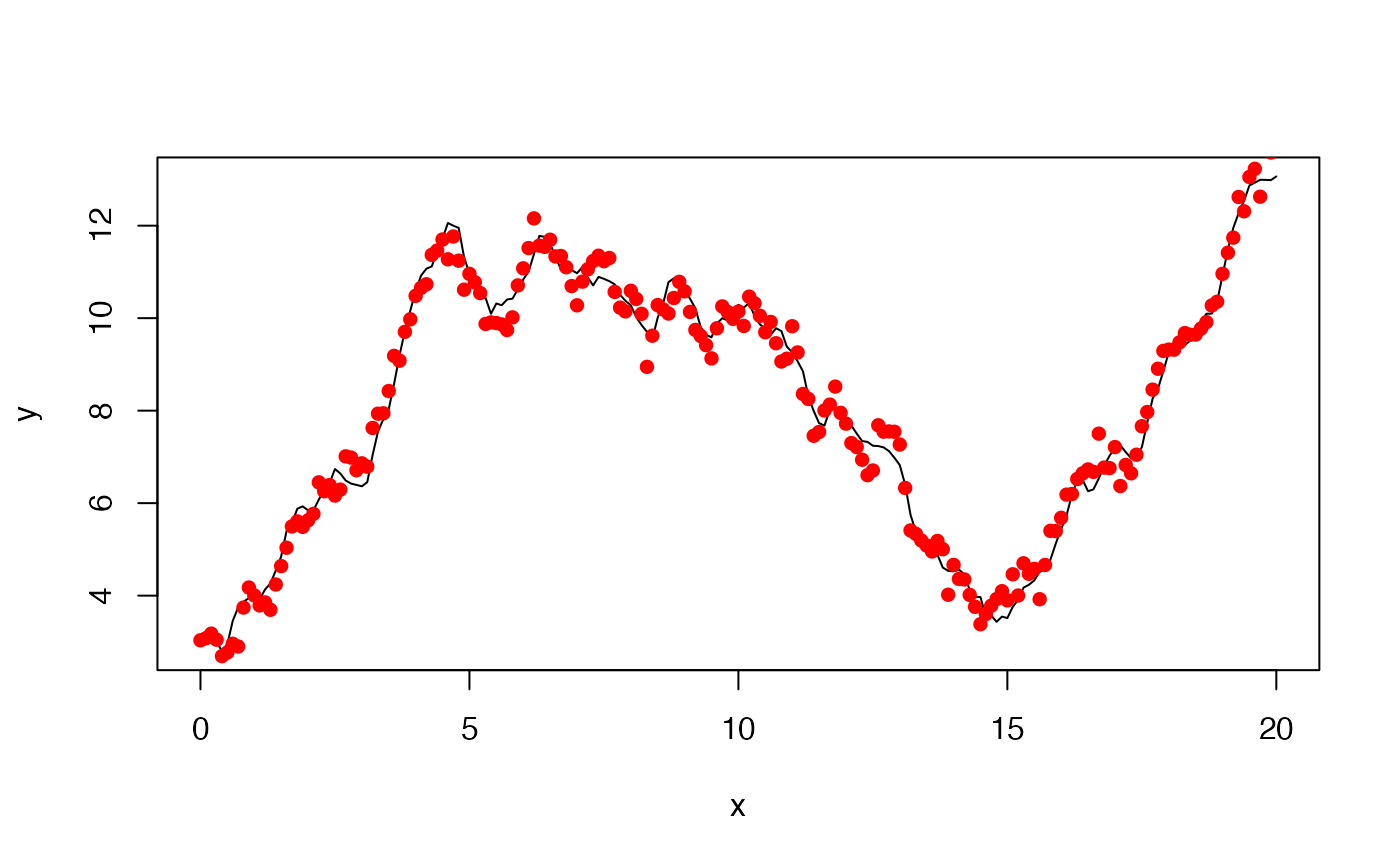
# plot the k.ahead=10 predictions
plot(pred, against="y.data")



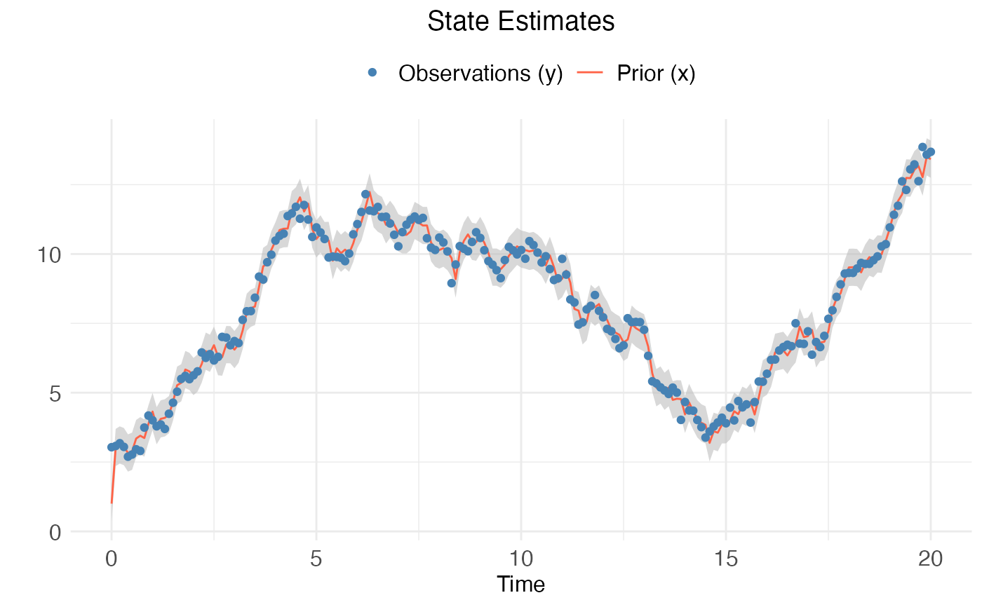
# plot filtered states
plot(fit, type="states", against="y")